Introduction:

Various industries are adopting this culture in the modern data-driven environment. For this culture, data preprocessing and dimensionality reduction are crucial steps in ensuring the efficiency, accuracy, security, and privacy of building AIML-powered applications.

With the exponential growth of data, traditional techniques have been enhanced with unique innovations to handle challenges such as quality, redundancy, and high dimensionality, which has become a high-demand activity.

This article explores cutting-edge advancements in Data Preprocessing and Dimensionality Reduction techniques, highlighting their impact on computational performance and helping to enrich predictive accuracy.

Traditional Data Preprocessing Techniques

Traditional data preprocessing techniques are very familiar to everyone and include data cleaning, integration, transformation, and reduction based on the requirements. Generally, all these exercises are aimed at preparing raw data for analysis or machine learning models. From an industry point of view, this is the so-called “GOLDEN DATA SET.”

Let's discuss the techniques mentioned above:

Data Cleaning is the process of removing noise from the data, such as duplicates, missing values, outliers, and other inconsistencies.

• Handling Missing Values: This is a significant issue when collecting data from a source. So, we must carefully deal with missing data points by replacing them with a mean, median, or mode. This process is technically called IMPUTATION. In some situations, the row will be removed from the dataset and made neat.
• Removing Noise and Outliers: We must do the proper exercise to Identify and address data inconsistencies. In some situations, the values significantly deviate from the norms and are unrealistic. This can be removed from the dataset by a straight removal process after getting approval from data owners. - Business Stakeholders
• Data Consistency: For AIML model building, we must ensure that the data is formatted and structured consistently as per business rules such as email ID, phone number, etc.,

Data Integration: This is a key process in the Data Engineering portfolio; because the data from the source cannot meet our expectations, we have to apply business rules and conditions to make them usable versions from the source. Here, the ETL or ELT process plays a vital role.

• Combining Data from Multiple Sources: Integrating data from different tables or files into a unified dataset to accompany the data analytics, science and AIML expectations.
• Data Transformation: Converting data to a standard format or structure based on data-driven solutions. We have to Identify and resolve inconsistencies in the structure and naming of data from different sources, which is a significant task.

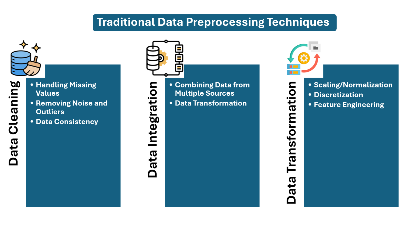
Data Transformation: This process involves various forms of data transformation, such as normalisation and feature engineering.

• Scaling/Normalisation: Transforming numerical data to a specific range (e.g., 0-1) or standard deviation, mean, median, or mode if any data imbalance symptoms exist in the dataset.
• Discretisation: In most situations, the nature of the data cannot be helpful for data-driven aspects, so converting continuous data into discrete or categorical values depends on the scenarios.
• Feature Engineering: In some situations, we create new features or transform existing ones into new and valuable ones. This could be feature creation, merging, or merging to improve model performance. Primary, such features don't come along with data sources.

We have discussed traditional data processing techniques so far. Now, let's explore how advanced techniques are used.

Advanced-Data Preprocessing Techniques

Advanced data preprocessing techniques go beyond the traditional techniques that we discussed earlier. Advanced data processing for data-driven solutions is required to enhance data quality, improve model performance, and handle complex data structures innovatively. These techniques leverage machine learning, deep learning, statistical methods and automated feature engineering to transform raw data into a more structured and usable format for analysis. These methods are essential in real-time applications such as healthcare, finance, cybersecurity, and manufacturing to improve decision-making and performance.

Here is a List of Key Advanced Data Preprocessing Techniques

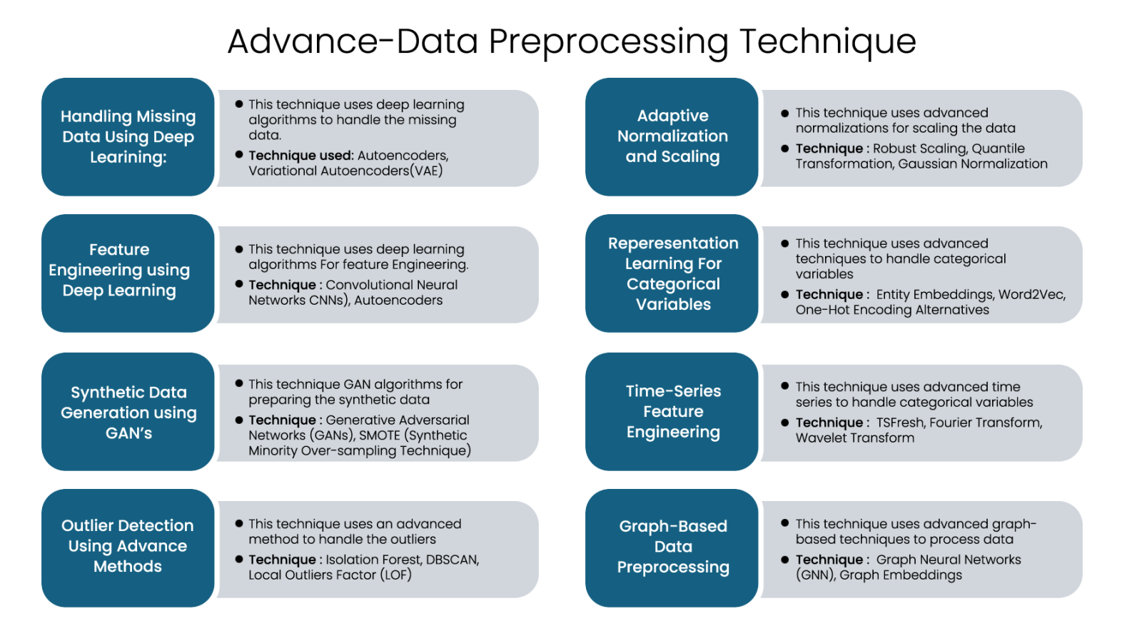
Handling Missing Data Using Deep Learning: This technique uses deep learning algorithms to handle the missing data. Techniques used: Autoencoders, Variational Autoencoders (VAE)

• Autoencoders: This technique is a category of neural network that learns a compressed representation of data and recreates it while filling in missing values.
• Variational Autoencoders (VAE): This technique adopts a probabilistic approach to generating the missing values by learning the underlying space representations from the given dataset.

Advantages of Using Autoencoders for Missing Data

• More Accurate: Learns data distribution instead of simple mean imputation.
• Preserves Relationships: Keeps feature dependencies intact.
• Handles High-Dimensional Data: Works well with large datasets.

Autoencoders Implementation for Handling Missing Data

#import required libraries

import numpy as np

import pandas as pd

from tensorflow.keras.models import Model

from tensorflow.keras.layers import Dense, Input

from sklearn.impute import SimpleImputer

from sklearn.preprocessing import MinMaxScaler

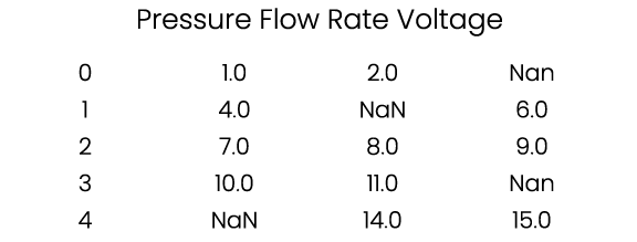
#Defining a simple array to build the dataset with null values

data = np.array([

[1, 2, np.nan],

[4, np.nan, 6],

[7, 8, 9],

[10, 11, np.nan],

[np.nan, 14, 15]

])

#Features for the above data

df = pd.DataFrame(data, columns=['pressure', 'flow_rate', 'voltage'])

print("Original Data with Missing Values:\n", df)

# Implementing SimpleImputer as a mean

#implementing transformation

imputer = SimpleImputer(strategy='mean')

data_imputed = imputer.fit_transform(df)

# Normalize data for better training performance after transform

scaler = MinMaxScaler()

data_scaled = scaler.fit_transform(data_imputed)

# Define the input shape

input_dim = data_scaled.shape[1]

# Encoder implementation

input_layer = Input(shape=(input_dim,))

encoded = Dense(8, activation='relu')(input_layer)

encoded = Dense(4, activation='relu')(encoded)

# Decoder implementation

decoded = Dense(8, activation='relu')(encoded)

decoded = Dense(input_dim, activation='linear')(decoded) # Output layer reconstructs input

# Define the Autoencoder model

autoencoder = Model(input_layer, decoded)

autoencoder.compile(optimizer='adam', loss='mse')

# Train the Autoencoder

autoencoder.fit(data_scaled, data_scaled, epochs=300, batch_size=2, verbose=0)

# Predict the reconstructed data

reconstructed_data = autoencoder.predict(data_scaled)

# Reverse scaling to original data range

reconstructed_data = scaler.inverse_transform(reconstructed_data)

# Convert back to DataFrame

df_imputed = pd.DataFrame(reconstructed_data, columns=['pressure', 'flow_rate', 'voltage'])

print("Imputed Data Using Autoencoder:\n", df_imputed)

1/1 ━━━━━━━━━━━━━━━━━━━━ 0s 91ms/step

Imputed Data Using Autoencoder:

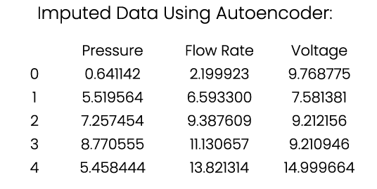
If you look at how the missing values are filled with 'mean' using Autoencoder.

Outlier Detection Using Advanced Methods

Outlier detection is a big challenge in data-driven solutions. DBSCAN (Density-Based Spatial Clustering of Applications with Noise) and LOF(Local Outlier Factor) are powerful unsupervised techniques for detecting outliers, specifically for high-dimensional data. These techniques help identify anomalous data points that do not conform to the general distribution in the given dataset.

Let's try to implement these techniques on a simple dataset with outliers.

Python code for DBSCAN-Based Outlier Detection

#import required libraries

import numpy as np

import pandas as pd

import matplotlib.pyplot as plt

from sklearn.cluster import DBSCAN

from sklearn.preprocessing import StandardScaler

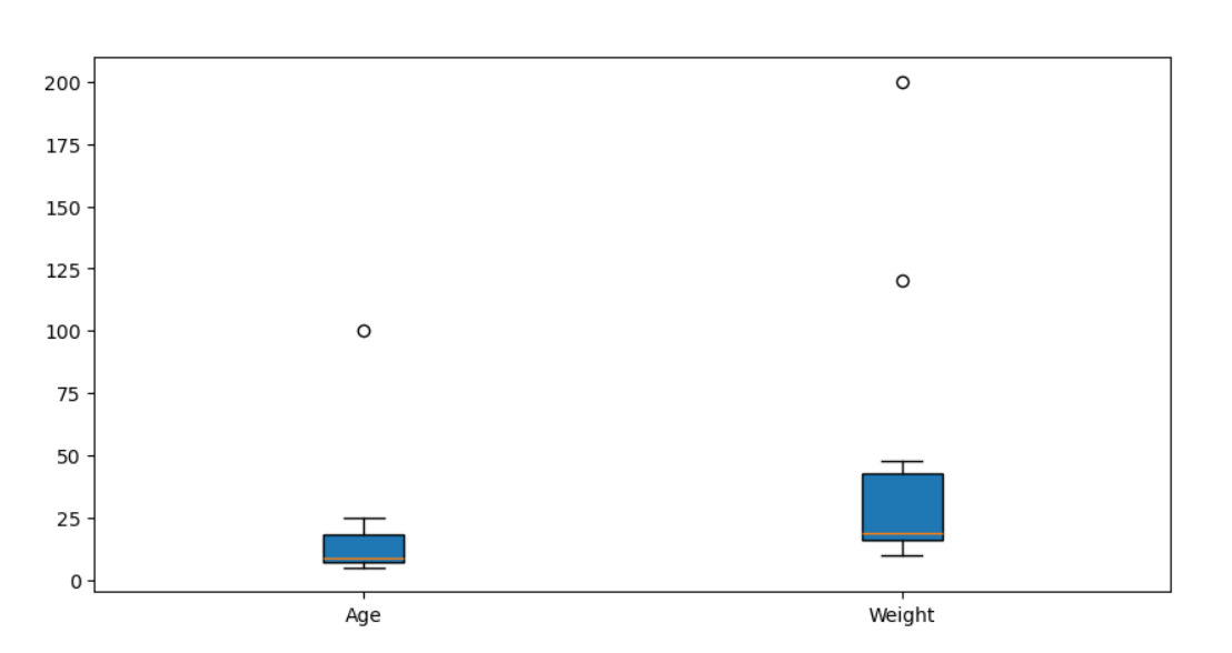
# sample dataset with Age (Years) and Weight (kg) for our analysis

data = np.array([

[5, 10], [7, 12], [13, 20], [18, 37], [18, 48], [25, 120], # Outlier at (25, 120)

[7, 15], [7, 17], [8, 19], [9, 18], [100, 200] # Extreme outlier (100, 200)

])

#Features

df = pd.DataFrame(data, columns=['Age', 'Weight'])

# Normalize the dataset using StandardScaler (DBSCAN is sensitive to scale differences)

scaler = StandardScaler()

data_scaled = scaler.fit_transform(df)

# Apply DBSCAN with optimised parameters for Age and Weight

eps_value = 1.2 # Based on data distribution (distance threshold)

min_samples_value = 3 # Minimum points needed for a cluster

#applying DBSCAN

dbscan = DBSCAN(eps=eps_value, min_samples=min_samples_value)

df['Cluster'] = dbscan.fit_predict(data_scaled)

# Marking outliers by assigning DBSCAN assigns -1 to noise points

df['Outlier'] = df['Cluster'] == -1

#print the Outliers

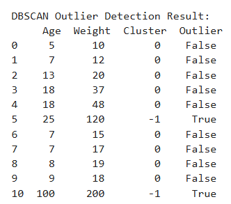
print("\nDBSCAN Outlier Detection Result:\n", df)

Output

DBSCAN Outlier Detection Result:

 

Innovations in Dimensionality Reduction

Dimensionality reduction techniques help reduce the number of features in a given dataset to improve model efficiency and reduce overfitting challenges. They preserve important information, avoid losing any features, avoid the feature engineering process timeline, apply statistical methods, and significantly reduce the features.

Innovative dimensionality reduction techniques are available to handle this process; below are the key techniques.

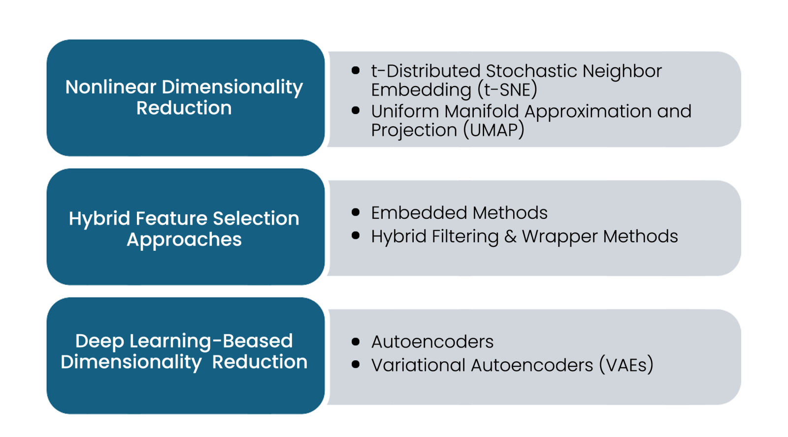
Nonlinear Dimensionality Reduction: When traditional PCA methods cannot effectively capture data using linear methods, nonlinear dimensionality reduction techniques are used, specifically when data has highly complex and nonlinear structures.

• t-Distributed Stochastic Neighbor Embedding (t-SNE): it helps visualise high-dimensional datasets by preserving structure while reducing the dimensions of the given dataset.
• Uniform Manifold Approximation and Projection (UMAP): This technique is highly scalable and faster than t-SNE, preserving local and global structures in lower dimensions.

Deep Learning-Based Dimensionality Reduction: Powerful deep learning-based dimensionality reduction techniques are available, which are listed below.

• Autoencoders:These are NN (Neural network)- based autoencoders that compress high-dimensional datasets into meaningful lower-dimensional datasets
• Variational Autoencoders (VAEs):These advanced models learn from probabilistic latent space representations and are best suited for complex datasets. They also improve dimensionality reduction at a high rate.

 

Hybrid Feature Selection Approaches: This technique combines multiple feature selection methods, reduces dataset dimensionality, and maintains the model's predictive power. It has been proven in many cases.

• Embedded Methods: This method integrates feature selection into the model training process, using techniques such as Lasso regression and decision tree-based methods.
• Hybrid Filtering & Wrapper Methods: This wrapper-based approach combines statistical filtering with enhanced feature selection approaches.

 

Conclusion

We have discussed the evolution of data preprocessing and dimensionality reduction techniques and how they are shaping the future of machine learning and improving computational efficiency and model performance. We explored and experimented with automated data cleaning, synthetic data processing, deep learning-based feature selection, and hybrid dimensionality reduction techniques, transforming how data is handled. Future directions include highly innovative methods such as quantum computing for data preprocessing by leveraging quantum algorithms for faster preprocessing and dimensionality reduction of datasets and federated learning for privacy-preserving data preprocessing, which allows the decentralised data preprocessing without compromising user privacy and security. With all these advancements, data-driven applications will continue to grow and make machine-learning models more accurate and efficient.