Simple linear regression is used to find out the best relationship between a single input variable (predictor, independent variable, input feature, input parameter) & output variable (predicted, dependent variable, output feature, output parameter) provided that both variables are continuous in nature. This relationship represents how an input variable is related to the output variable and how it is represented by a straight line.

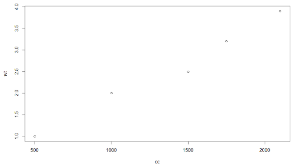
To understand this concept, let us have a look at scatter plots. Scatter diagrams or plots provides a graphical representation of the relationship of two continuous variables.

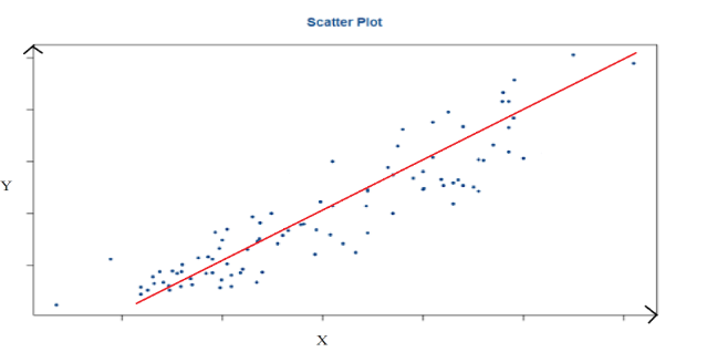
After looking at scatter plot we can understand:

1. The direction
2. The strength
3. The linearity

The above characteristics are between variable Y and variable X. The above scatter plot shows us that variable Y and variable X possess a strong positive linear relationship. Hence, we can project a straight line which can define the dаta in the most accurate way possible.

If the relationship between variable X and variable Y is strong and linear, then we conclude that particular independent variable X is the effective input variable to predict dependent variable Y.

To check the collinearity between variable X and variable Y, we have correlation coefficient (r), which will give you numerical value of correlation between two variables. You can have strong, moderate or weak correlation between two variables. Higher the value of “r”, higher the preference given for particular input variable X for predicting output variable Y. Few properties of “r” are listed as follows:

1. Range of r: -1 to +1
2. Perfect positive relationship: +1
3. Perfect negative relationship: -1
4. No Linear relationship: 0
5. Strong correlation: r > 0.85 (depends on business scenario)

Command used for calculation “r” in RStudio is:

> cor(X, Y)

where, X: independent variable & Y: dependent variable Now, if the result of the above command is greater than 0.85 then choose simple linear regression.

If r < 0.85 then use transformation of dаta to increase the value of “r” and then build a simple linear regression model on transformed dаta.

Steps to Implement Simple Linear Regression:

1. Analyze dаta (analyze scatter plot for linearity)
2. Get sample dаta for model building
3. Then design a model that explains the dаta
4. And use the same developed model on the whole population to make predictions.

The equation that represents how an independent variable X is related to a dependent variable Y.

Example:

Let us understand simple linear regression by considering an example. Consider we want to predict the weight gain based upon calories consumed only based on the below given dаta.

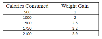
Now, if we want to predict weight gain when you consume 2500 calories. Firstly, we need to visualize dаta by drawing a scatter plot of the dаta to conclude that calories consumed is the best independent variable X to predict dependent variable Y.

We can also calculate “r” as follows:

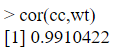
As, r = 0.9910422 which is greater than 0.85, we shall consider calories consumed as the best independent variable(X) and weight gain(Y) as the predict dependent variable.

Now, try to imagine a straight line drawn in a way that should be close to every dаta point in the scatter diagram.

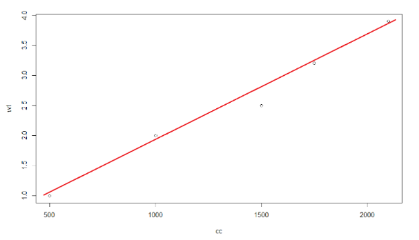
To predict the weight gain for consumption of 2500 calories, you can simply extend the straight line further to the y-axis at a value of 2,500 on x-axis . This projected value of y-axis gives you the rough weight gain. This straight line is a regression line.

Similarly, if we substitute the x value in equation of regression model such as:

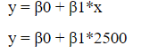
y value will be predicted.

Following is the command to build a linear regression model.

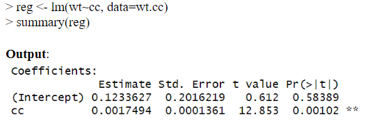
We obtain the following values

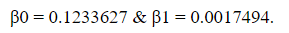
Substitute these values in the equation to get y as shown below.

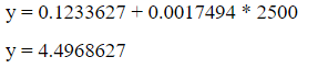
So, weight gain predicted by our simple linear regression model is 4.49Kgs after consumption of 2500 calories.